Thermal curing is the process of temperature-induced chemical change in a material, such as the polymerization of a thermoset resin. This process is relevant, for example, when a precursor resin is heated and hardens during the manufacturing of composites. You can often assume that the material does not flow during curing, which simplifies the analysis. Thermal curing is very easy to model within the core functionality of COMSOL Multiphysics, as we will show in this blog post.
The Thermal Curing Process
Thermosets are a class of polymer materials that undergo an irreversible chemical reaction, causing the polymer chains to cross-link and form a rigid material. This chemical reaction can be due to heat, light, or the addition of a chemical catalyst. Bakelite, one of the first thermosets, is often credited as kicking off the polymer industry. Bakelite is a very hard material that is resistant to many chemicals, is a good electrical insulator, and has an attractive surface finish. The material was used in a variety of early consumer products, such as telephones and radio cabinets.

A Bakelite radio cabinet. Image by Joe Haupt — Own work. Licensed under CC BY-SA 2.0, via Wikimedia Commons.
Bakelite and other thermosets come in various precursor forms, such as powders and thick viscous liquids. These precursors are put into a mold and heated under high pressure. Additional filler materials are often added to improve the properties of the final product. Carbon fiber and fiberglass composites, for example, bond relatively strong but flexible fibers together using a relatively rigid thermoset matrix.
Now, depending upon the exact manufacturing process, the precursor material might not move around or flow significantly during the curing step. If this is so, then you can develop a very simple model to predict the curing based upon the temperature. Let’s now look at how to implement such a model in COMSOL Multiphysics.
Modeling Thermal Curing in COMSOL Multiphysics
We will look at simulating curing during a transfer molding process, wherein the material is loaded into a mold and then heated, as shown in the schematic below. During heating and curing, the material does not move around inside the mold, and for simplicity, we won’t consider any filler materials. A thin-walled part, such as the radio cabinet shown earlier, can be reasonably modeled with a one-dimensional model through the thickness. Since the material is heated uniformly and at a known rate on both sides, we can exploit symmetry to only model one half of the material.
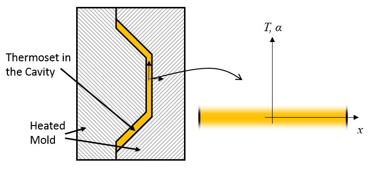
Schematic of a mold with a thermoset curing inside and the equivalent model for temperature and degree of cure.
Our model will compute the variation in time of the temperature, T, and the degree of cure, \alpha, of the thermoset from the centerline to the mold wall. Assuming no flow, the equation governing heat transfer in the thermoset precursor is:
(1)
where \rho, C_p, and k are the density, specific heat, and thermal conductivity of the material.
The degree of cure is \alpha and as the material cures, it absorbs heat, thus there is a negative volumetric heat source that is a function of H_r, the heat of the reaction. The rate of change of the degree of cure is often described by:
(2)
where the Arrhenius equation defines the temperature-dependent reaction rate, with A being the frequency factor, E_a being the activation energy, R as the universal gas constant, and n as the order of the reaction.
Let’s now look at how to set up this model in COMSOL Multiphysics, starting with the definitions of a few Global Parameters defining the properties of our representative thermoset material.
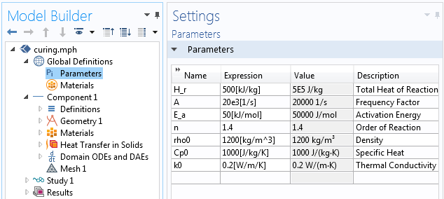
The Global Parameters define a set of representative material properties of a thermoset.
Our modeling domain is simply a 5-mm-long 1D interval, with the material properties as shown above. The Heat Transfer in Solids interface solves for the temperature distribution over time, starting with the specified initial temperature along with a Thermal Insulation boundary condition on one end. A Heat Flux boundary condition at the other end of the domain applies 10 kW/m2 due to the heating of the mold.
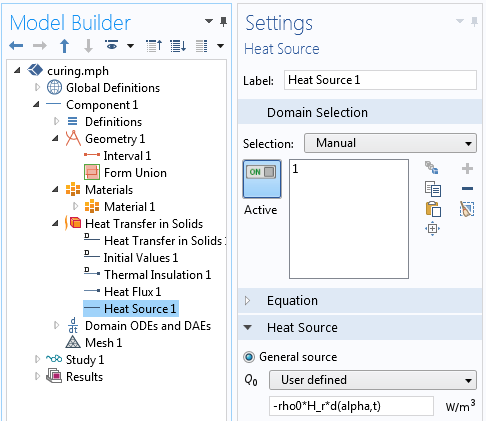
The absorption of heat due to the material curing is modeled via the Heat Source feature.
The endothermic effect of the curing is accounted for via a volumetric heat source, -rho0*H_r*d(alpha,t), as shown above. This feature implements the right-hand term from Equation 1 based upon the time derivative of the degree of cure.
We now need to add one more interface to solve for the degree of cure, and this is done via the Domain ODEs and DAEs interface, as shown below. Note that the field name is alpha. Pay special attention to how the units are set up.
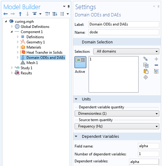
Settings for the Domain ODEs and DAEs interface, which solves for the degree of cure.
Lastly, looking at the settings for the Distributed ODE feature, we see that the Source Term is A*exp(-E_a/R_const/T)*(1-alpha)^n and the Damping term is unity, while the Mass Coefficient is zero, thus giving us Equation 2. An initial condition of zero means that the material is modeled starting from the uncured state.
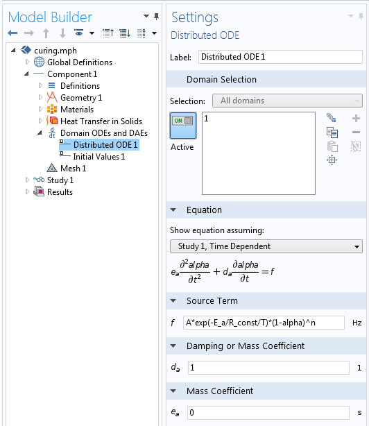
Settings for the Distributed ODE feature that solves for the degree of cure.
And that’s all there is to it: We can solve our model for a ten-minute curing time and plot the temperature and degree of cure through the thickness and at the inside and midpoint of the material, as shown below. Here, we apply a constant heat load at one side, so we will want to check the maximum temperature and the degree of cure through the thickness.
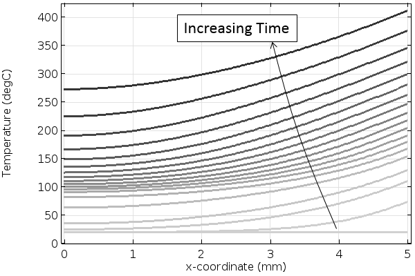
The temperature increases through the thickness of the material over time. Darker lines indicate increasing time.
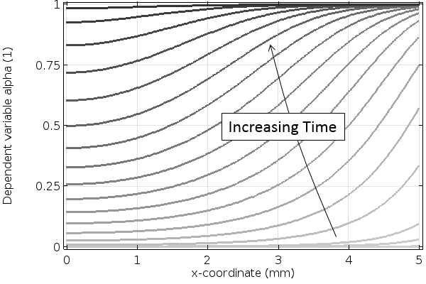
The degree of cure through the material over time. Darker lines indicate increasing time.
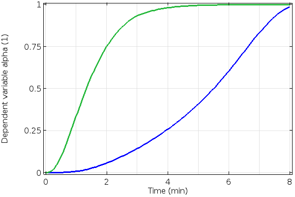
The degree of cure at the center (blue) and side (green) of the thermoset material.
Closing Remarks and Further Reading on Thermal Curing
We have shown how to quickly set up a thermal curing model entirely within the core capabilities of COMSOL Multiphysics. Of course, you can use a similar approach if you want to model the curing of other materials, such as concrete. If the material curing is due to light, such as in a photopolymerization process, you may also want to look over the various ways of modeling the interaction of light with materials, and in particular the modeling of light being absorbed within the volume of a solid as governed by the Beer-Lambert law.
The model presented here can be easily extended in many ways, including adding temperature nonlinearities to all of the materials properties, incorporating the effect of a filler material, and solving these equations in a 3D model. If you would like to see work that includes these examples, please read:
- T. Behzad and M. Sain, “Finite element modeling of polymer curing in natural fiber reinforced composites“, Composite Science and Technology, vol. 67, pp. 1666-1673, 2007.
If you have other questions or are interested in using COMSOL Multiphysics for your thermal curing modeling needs, please contact us.