Whenever solid materials are heated enough, they will melt and then vaporize to a gas. Certain materials will even go directly from the solid to the gas phase, a process referred to as sublimation or ablation. If the material is heated strongly enough, there will be significant material removal. Today, we will look at how you can model this process in COMSOL Multiphysics.
Material Removal by Ablation
As a solid material is heated, its temperature will rise and it will eventually undergo a phase transition. This transition can involve either going to the liquid phase and then to the gas phase or going directly to the gas phase. For our purposes, we will consider only those materials that go directly to the gas phase.
Let’s further assume in this case that the material is being heated in such a way that the maximum temperature develops on the surface and that there is no internal heating that might lead to an internal gas-filled void within the solid. Thus, we limit ourselves to situations where sublimation occurs at the surface. We can also assume that once the material transitions to the gas phase, it is no longer thermally significant. This is a reasonable assumption whenever there is some kind of additional surrounding gas flow that carries the vaporized material away. The process of heating the surface of a material to the gaseous state and quickly removing the gas from the vicinity of the solid is often called ablation.
Ablation requires a large heat flux to be delivered to the surface of the material. One of the most practical examples of such a heat source is a laser. This approach is applied to a range of processes, including laser machining, surgical procedures, and laser engraving, among others. The heat source, of course, does not necessarily need to be a laser. In fact, ablative heat shields have been used to help spacecraft survive the high heat loads experienced during atmospheric reentry.

An artist’s rendition of a heat shield on a reentry vehicle.
Modeling ablation requires setting up and solving a model that computes the temperature variation in a solid material over time, while also including the heat of sublimation and the resultant material removal. First, we must develop a thermal boundary condition that enforces the condition that the solid material cannot exceed the sublimation temperature. Second, we need to develop a method for modeling the mass removal from the domain of interest. Let’s see how we can accomplish these tasks in COMSOL Multiphysics.
Modeling Thermal Ablation in COMSOL Multiphysics
To begin, we’ll consider a highly simplified model of the heat shield on the spacecraft shown above. We will assume that the heat flux across the heat shield is uniform in time and space. Another assumption we make is that the material properties of the heat shield are constant and that there are negligible temperature gradients in the plane of the shield as compared to through the thickness. Under these assumptions, we can reduce our model to a one-dimensional domain, as illustrated below.
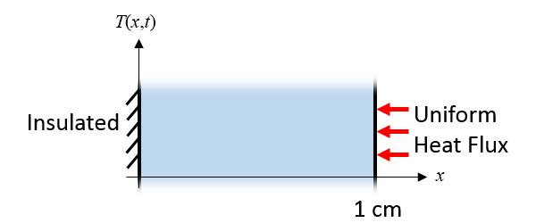
A heat shield (as pictured earlier) with a uniform heat flux can be reduced to a 1D model.
Our thermal boundary conditions for the 1D domain begin with the thermal insulation condition at one side, meaning that there is no removal of heat through the spacecraft body. At the other side, there is a uniform constant heat flux that approximates the effect of atmospheric heating during reentry.
Lastly, we need to include a set of boundary conditions that model the heat loss due to material ablation. As the material reaches its ablation temperature, it changes its state to a gas and is removed from our modeling domain. Therefore, the solid material cannot become hotter than the ablation temperature, and when the material is at its ablation temperature, there is a loss of mass from the surface that is governed by the material density and the heat of sublimation. To model this element, we will need both a thermal boundary condition and a way to model the material removal.
The thermal boundary condition that we will introduce to model ablation is an ablative heat flux condition of the form:
(1)
where q_a is the heat flux due to material ablation, T_a is the ablation temperature, and h_a=h_a(T) is a temperature-dependent heat transfer coefficient that is zero for T < T_a and increases linearly as T > T_a.
The slope of this curve is very steep, enforcing that the temperature of the solid cannot markedly exceed the ablation temperature. In addition to the thermal boundary condition, we must also include the material removal. The rate at which the solid boundary is eroded is:
(2)
where v_a is the material ablation velocity, \rho is the material density, and H_s is the heat of sublimation.
Let’s now look at how these equations are implemented in COMSOL Multiphysics, starting with the material properties and heat load, as defined via the Global Parameters shown below.
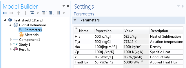
The Global Parameters applied to our 1D model.
Next, the Ramp function is used to define the temperature-dependent heat transfer coefficient needed in Equation (1), as illustrated in the following screenshot. The slope itself is arbitrary, but too small of a value will cause the ablation temperature to be exceeded and too large of a value will cause slow numerical convergence.
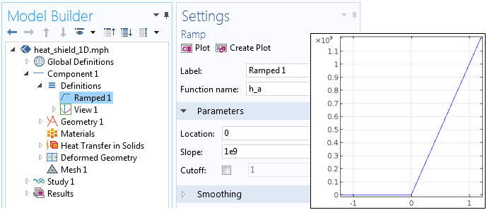
The Ramp function has a very steep slope.
Our model consists of a 1D domain that is 1 cm long. The Heat Transfer in Solids interface is used to model the temperature evolution over time. The incident heat flux is applied at one side and the thermal insulation condition is applied at the other side. The ablative heat flux of Equation (1) is implemented as shown in the screenshot below. Since heat flux conditions contribute, it is the sum of the incident heat flux and the ablative heat flux that is applied to the boundary.
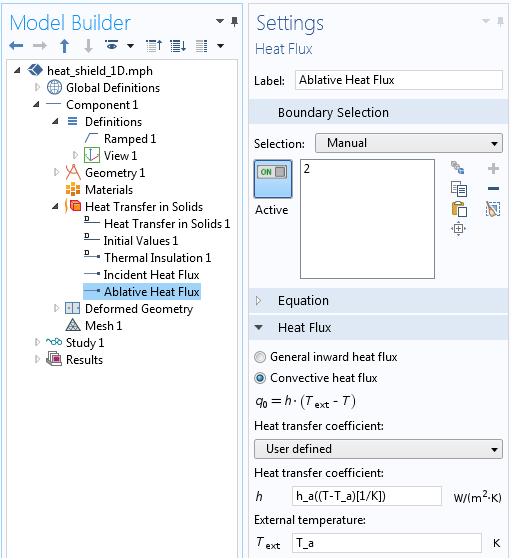
The implementation of the ablative heat flux condition from Equation (1).
To model the material removal, the Deformed Geometry interface is used. The Free Deformation feature allows the domain to change in size, as prescribed by the boundary conditions. On one side (the insulated side), a prescribed deformation enforces no displacement of the boundary. On the other end of the domain, the Prescribed Normal Mesh Velocity condition enforces Equation (2), the material removal rate, as depicted below.
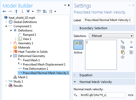
The implementation of the material removal in Equation (2), using the Deformed Geometry interface.
The mesh velocity is given by the expression ht.hf2.q0/(rho*H_s), where ht.hf2.q0 is the heat flux computed via the Ablative Heat Flux boundary condition that was earlier defined. You can always find the definitions of all such internally defined COMSOL variables by going to Results > Reports > Complete Report.
With those features, we have included the effect of ablation and can solve our model for the temperature evolution over time, as plotted below. We can observe that the temperature at the right side of the solid rises up to the ablation temperature and the material starts to become removed from the domain. As the material is ablated, the temperature at the boundary is maintained. Additionally, note that the derivative of the temperature, with respect to position, changes once the material starts to ablate, indicating that the total heat flux has changed.
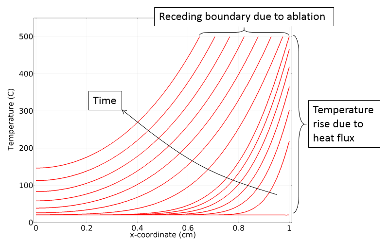
The temperature evolution over time in the 1D domain.
Let’s finish up our discussion by showing the results from a somewhat more complicated problem. The problem involves an axisymmetric geometry with a heat load that has a Gaussian intensity profile. Our focus is simulating laser heating and ablating the material to machine a hole. We can use the exact same model setup as described above, but on a 2D domain.
The simulation results, highlighted in the following animation, show the hole forming over time. The domain change is significant so, in this example, the Deformed Geometry interface uses a Hyperelastic smoothing type to deform the mesh. Note that the Deformed Geometry interface does not admit any topological changes to the domain. Therefore, we cannot model the formation of a through-hole, only the material removal from one side of the modeling domain.
An animation showing laser ablation in a 2D axisymmetric model.
Closing Remarks on Modeling Thermal Ablation
In today’s blog post, we have demonstrated how to use a Heat Flux boundary condition and the Deformed Geometry interface with the Prescribed Mesh Velocity feature to model ablation of a material. The example presented has been kept as simple as possible to focus only on the modeling of ablation. A more realistic model would also include radiative heat transfer from the surface and temperature-dependent material properties.
Further, it is possible to consider a pulsed heat load, a common element in laser machining. To learn more about modeling such cases, please have a look at this earlier blog entry. When heating with a laser, it is also possible for the light to be penetrated some finite distance into the material. In such a case, you may be able to use the Beer-Lambert law to model the energy deposition, among other methods for modeling the laser heating of materials.
If the material itself first undergoes some chemical changes during the heating, we encourage you to read through our previous blog post on the modeling of thermal curing. You can also consider ablation of a thin thermally insignificant layer by following a different approach of introducing an additional equation to track the material damage.
If you’re interested in modeling thermal ablation with COMSOL Multiphysics or have any other questions regarding these topics, please don’t hesitate to contact us.