Have you ever wanted to quickly predict the temperature of an enclosed structure, such as your house, that is exposed to ambient environmental conditions? The temperature inside depends on the surrounding air temperature, wind speed, and solar loads, all of which have significant variability. For simplicity, we often also want to approximate the inside air as well-mixed. Today, we will discuss the tools in COMSOL Multiphysics that help you quickly build such thermal models.
Approximating the Air Flow Inside and Around Your House
Let’s say that you want to quickly predict the temperature of an enclosed structure that is exposed to ambient conditions. This could be a small structure, such as a junction box on a utility pole or a shipping container, or perhaps a structure that is familiar to all of us: a house.
To begin, we can consider a small house, as illustrated below. The house features four walls, a roof, one big room, a door, and a few windows. We will assume that there is a fan that causes the air inside to be reasonably well-circulated, meaning that if we measure the air temperature at any one point inside, it will be the same as it is at any other point inside the room. This is a very good approximation of what happens if we have a mixing ventilation system.
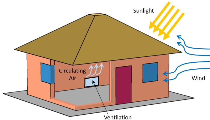
A very simple model of a house. We are interested in the temperature inside the structure.
Since the air is well-circulated, we only need to solve for a single spatially uniform air temperature. This room air temperature varies over time due to the air conditioning and heating, along with heat transfer through the walls. At the outside of the walls, we also need to apply thermal boundary conditions to reflect the ambient air temperature, wind speed, and solar heat loads.
Now we all know that weather is notoriously unpredictable. Therefore, rather than trying to build a thermal model of the environment around our house, we instead look to historical weather data. The American Society of Heating, Refrigerating, and Air-Conditioning Engineers compiles a database of information gathered at weather stations located around the world. In COMSOL Multiphysics® version 5.2a, this tabulated data is now available as input for simulations in COMSOL Multiphysics.
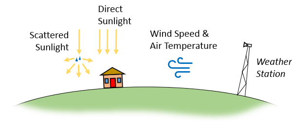
A weather station records direct and scattered solar irradiance, wind speed, and air temperature.
The tabulated meteorological data includes the historical data for over 6000 different weather stations spanning the globe. Temperature, dew point, wind speed, air pressure, and direct and diffuse solar irradiation as a function of calendar day and time are available. Direct solar irradiation refers to the radiation that comes directly from the sun, while diffuse irradiance results from the scattering of direct sunlight through the particulates and clouds in the atmosphere. You can use the data from any nearby weather station as a reasonable estimation of the ambient conditions for your models. It is up to you to decide if you want to use the average, the average low or high, or the peak low or high temperature, dew point, and wind speed. Average high and average low are defined as the average plus or minus one standard deviation.
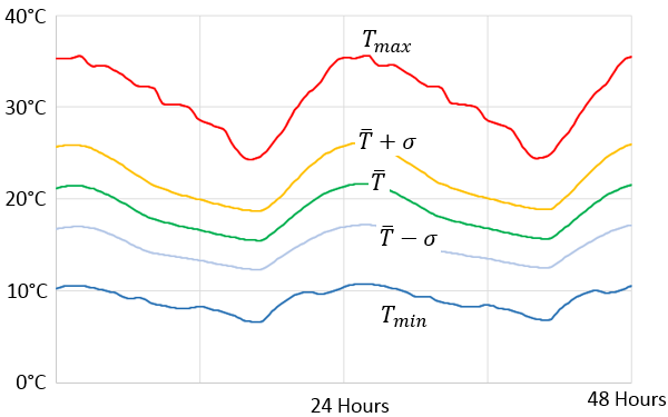
Sample plot of average, average high and low, and peak high and low temperature over two days.
Let’s now look at using such features within COMSOL Multiphysics to help us model the air inside our house and the ambient conditions outside.
Well-Mixed Air Inside a Room: Isothermal Domains
To model a well-mixed fluid domain like the air inside our house, we can use the Isothermal Domains feature available with the Heat Transfer Module. To use this feature, you first need to check the relevant check box in the Physical Model settings, as shown in the screenshot below.
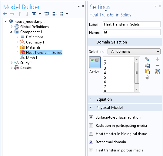
The “Isothermal domain” check box.
Once this functionality is enabled, you will be able to add Isothermal Domain features to the Heat Transfer interface, as depicted in the following screenshot. By default, this feature will compute the total mass and thermal heat capacity of the domain based on the assigned material properties. You can override these calculations with a user-specified domain mass and specific heat, if desired.
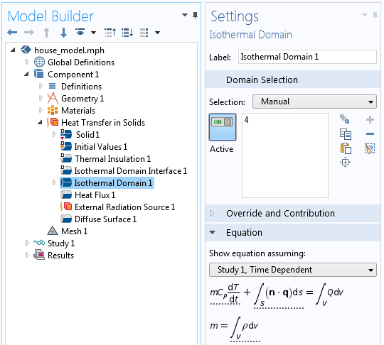
The Isothermal Domain interface.
The temperature variation of the isothermal domain over time is governed by the heat flux into and out of the domain through its boundaries. This is defined via the Isothermal Domain Interface boundary condition, which is illustrated in the screenshot below. You can specify one of several different conditions: Thermal Insulation, Continuity, Thermal Contact, Ventilation, or Convective Heat Flux. The last of these conditions, the Convective Heat Flux, is the most appropriate for describing the heat transfer between the average temperature of a well-mixed fluid domain and a solid domain.
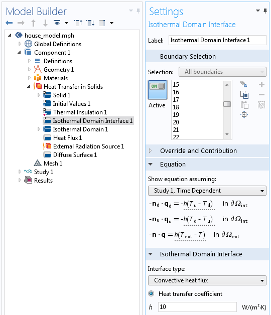
The boundary condition between an isothermal domain and surrounding domains.
Now that we have seen how to define a uniform air temperature within the house, let’s turn our attention outward, addressing the boundary conditions on the outside surfaces that are exposed to ambient conditions.
Tabulated Environmental Thermal Conditions: New Feature in COMSOL Multiphysics® Version 5.2a
The first step here is to choose the location of the weather station with the data that we want to use. This is handled in the settings for all of the heat transfer interfaces, as demonstrated below. You can choose from over 6000 different weather stations and select the date and time for the data that you want. By default, the software will update the time from the solver, so the ambient conditions will change if you are simulating for a long period of time.
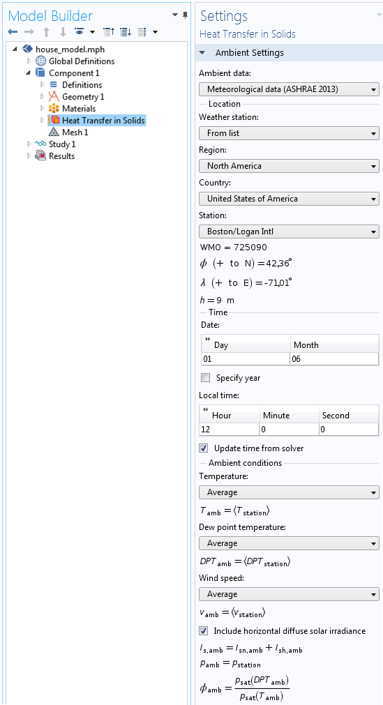
Screenshot showing how to define the ambient environmental data.
Once the location and time defining the ambient conditions are selected, the surrounding air temperature and wind velocity are defined and can be referenced from other features within the physics interface, such as the Heat Flux boundary condition.
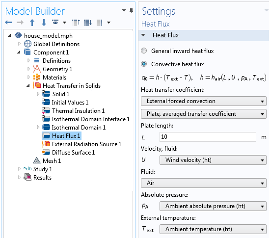
The ambient temperature, pressure, and wind speed are referenced by the Heat Flux boundary condition.
The ambient solar irradiance is used within the External Radiation Source feature, when using the Solar Position option, as highlighted below. Note that the ambient data contains the solar flux at noon under clear sky conditions. By entering the location and the time of day within this feature, the software will automatically recompute the orientation of the incident sunlight over the course of the day, as described in our earlier blog post on solar heating.
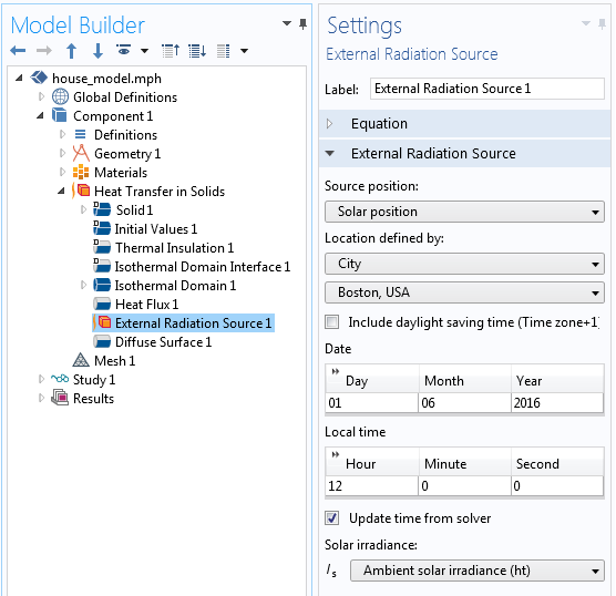
The ambient solar irradiance is an input for the External Radiation Source feature.
Now that we’ve seen all of the features that can be utilized, let’s take a look at some representative results. The animation below, for instance, plots the temperature over time and shows the incident direction of the solar flux.
Animation showing temperature and incident solar flux.
Further Possibilities for Thermal Modeling in COMSOL Multiphysics
Here, we have looked at a set of features that are useful for modeling structures that are exposed to ambient conditions and filled with well-mixed air. If you want to compute the airflow and air temperature variations within your structures, I encourage you to read our blog post “Modeling a Displacement Ventilation System“. You may also want to actively heat or cool your structures. For an introduction to this topic, take a look at my previous blog post “Implementing a Thermostat with the Events Interface“.
Say that you are further interested in modeling ventilation systems within larger buildings. If so, you will also want to consider the Pipe Flow Module, one of the add-on products to COMSOL Multiphysics. This video presentation offers further insight on modeling pipe flow for heating and ventilation.
We have not addressed the modeling of the walls here in detail. The model shown above simply treats the walls as uniform blocks of different materials. COMSOL Multiphysics is an ideal platform for performing a detailed analysis of the heat loss due to thermal bridging. Here are some example models that you can use to get started:
- Thermal Bridges in Building Construction — 3D Structure Between Two Floors
- Thermal Bridges in Building Construction — 3D Iron Bar Through Insulation Layer
- Thermal Bridges In Building Construction — 2D Square Column
- Thermal Bridges in Building Construction — 2D Composite Structure
- Parameterized Window and Glazing Preset Model
- Parameterized Window Preset Model
- Parameterized Roller Shutter Preset Model