When using the finite element method, we often want to model solid objects that are rotating and translating within other domains. The deformed mesh interfaces in COMSOL Multiphysics can be used to model these movements. In this blog post, we will look at the modeling of large linear translations and rotations of domains within other domains, while introducing efficient modeling techniques for addressing such cases.
Linear Translation of an Object Through a Domain
In a previous blog post, we discussed the modeling of objects translating inside of domains that are filled with a fluid, or just a vacuum. This initial approach introduced the use of the deformed mesh interfaces and the concept of quadrilateral (or triangular) deforming domains, where the deformation is defined via bilinear interpolation. Such a technique works well even for large deformations, as long as the regions around the moving object can be appropriately subdivided. This, however, is not always possible.
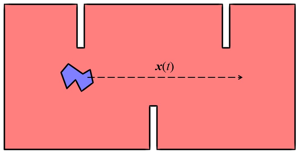
A solid object moving along a linear path inside of a complicated domain.
Consider the case shown above, where an object moves along a straight line path, defined by \mathbf x(t), through a domain with protrusions from the sides. In this situation, it would be quite difficult to implement the original approach. So what else can we do?
Using a Sliding Mesh for Large Linear Translations
The solution involves four steps. They are:
- Create several different geometric objects from our two domains
- Utilize the Form Assembly functionality to set up so-called identity pairs
- Define the linear movement with the previously developed mesh deformation techniques
- Use the identity pairs to ensure continuity in the physics that you are solving
We can begin by dividing our original model space into two different geometry objects, as depicted in the figure below. Here, the red domains represent the stationary domains and the blue domains represent the regions in which our object is linearly translating. The subdivision process takes place in the geometry sequence, which is then finalized with the Form Assembly operation.
For a description of this functionality and steps on how to use it, watch this video.
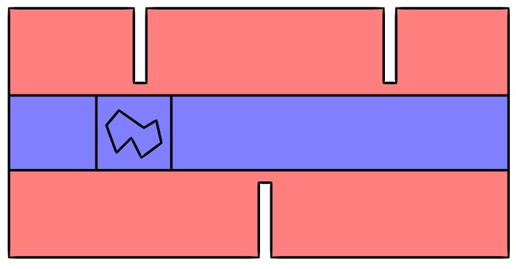
Subdividing the modeling space into different geometry objects.
The Form Assembly step will allow the finite element meshes in the blue domains to slide relative to the meshes in the red domains. This step will also automatically introduce identity pairs that can be used to maintain continuity of the fields for which we will be solving. Let’s take a look at a representative mesh that may be appropriate in this case.
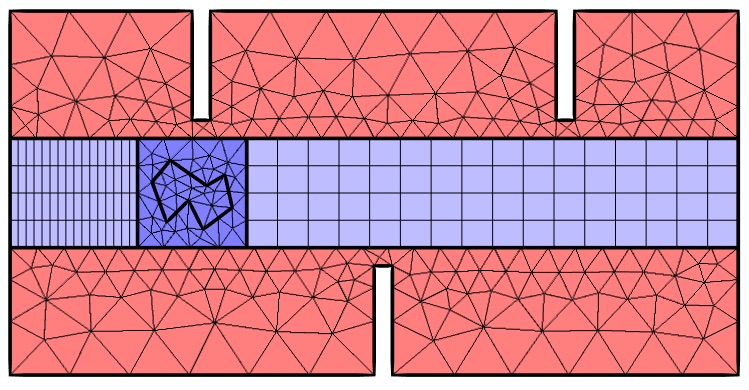
The subdivided domains with a representative mesh.
In the figure above, note that the dark red domains contain meshes that will not move at all. The dark blue domains, meanwhile, have translations completely defined by our known function, \mathbf x(t). The light blue domains are the regions in which the mesh will deform. We can simply use the previously introduced method of bilinear interpolation in these domains. You should also note that a Mapped mesh is used for these two rectangular domains and that the distribution of the elements is adjusted, such that they are reasonably similar in size or smaller than the adjacent nondeforming elements.
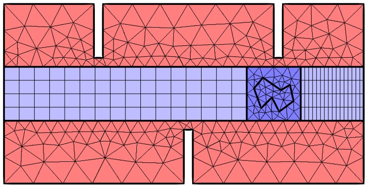
After the object has been linearly translated, the mesh in the light blue domains deforms.
Maintaining Solution Continuity
From the previous images, you can clearly see that the meshes no longer line up between the moving and stationary domains. While COMSOL Multiphysics version 5.0 has introduced greater accuracy in the handling of noncongruent meshes between domains, there are some things that you should be aware of when using this functionality.
As a result of the Form Assembly geometric finalization step, COMSOL Multiphysics will automatically determine the identity pairs — the mating faces at which the mesh can be misaligned. We simply need to tell each physics interface within our model to maintain continuity at these boundaries. This can be accomplished via the Pairs > Continuity boundary condition, which is available within the boundary conditions for all of the physics interfaces.
Once this feature is added and applied to all of the identity pairs, the software will apply additional conditions at these interfaces to ensure that the solution is as smooth as possible over the mesh discontinuity. Each identity pair has a so-called source side and a destination side. The mesh on the destination side should be finer in all configurations of the mesh.
Assembly meshes with noncongruent meshes at the boundaries can be used in combination with most physics interfaces. There are, however, a few important exceptions. Whenever you are solving an electromagnetics problem involving a curl operator on a vector field, such a technique cannot be used. Common physics interfaces that fall into this category include the 3D Electromagnetic Waves interfaces, the 3D Magnetic Fields interfaces, and the 3D Magnetic and Electric Fields interfaces. This still, of course, leaves us with a wide range of physics.
Let’s look at one case of computing the temperature fields around our object, with differing temperatures for the object and the surrounding domain’s outer walls. The contour plots of the temperature fields shown below verify that the solution is quite smooth over the boundary where the mesh is not continuous.
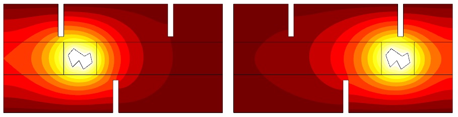
The temperature fields over time are smooth across the Continuity boundary condition applied to the identity pair.
Rotating the Object
At this point, you can probably already see how this same technique can be applied to a rotating object. We simply create a circular domain around our rotating object and use all of the same techniques we have discussed here. Of course, if the object is only rotating, we no longer need the deforming mesh — making things even a bit simpler for us.
The figures below show the same object from before, except now the object is rotating.
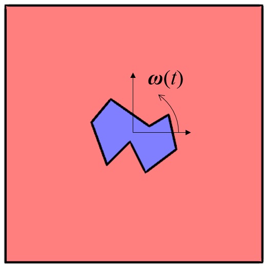
An object rotating about a point.
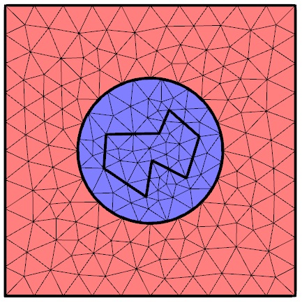
An assembly composed of stationary and rotating objects as well as the mesh.
The expressions for the prescribed deformation of the rotating domain, (X_{r}, Y_{r}), can be expressed in terms of the angular frequency, \omega; the undeformed geometry coordinates, (X_{g}, Y_{g}); the point about which the object is rotating, (X_{0}, Y_{0}); and time, t. This gives us the following expressions:
where the prescribed deformation in the Deformed Geometry interface is quite simply:
Seems easy, right? In fact, the technique outlined in this section is actually applied automatically in COMSOL Multiphysics when using the Rotating Machinery, Fluid Flow and the Rotating Machinery, Magnetic physics interfaces. This provides you with a behind-the-scenes look at what is going on within these interfaces!
Closing Remarks
We have now introduced methods for modeling the motion of solid objects inside fluid- or vacuum-filled domains. Although we have simply prescribed a displacement in all of these cases, the displacement of our solid objects could be computed and coupled to the field solutions in the surrounding regions. That is, however, a topic for another day.
Interested in learning more about using the deformed mesh interfaces for your modeling? Download the tutorial from our Application Gallery.