When designing and modeling devices such as chemical reactors, one of the quantities used to characterize the system is the residence time. This calculation is separate from the computation of the flow field, and can be done using the Particle Tracing Module. Let’s learn more…
Computing Residence Time and Other Factors
Let’s suppose that we are modeling a small flow cell, similar to a biosensor. We start with a fluid dynamics analysis, computing the flow of water around a set of obstructions. In this case, we can reduce the problem to a two-dimensional computational model, as shown in the image below.
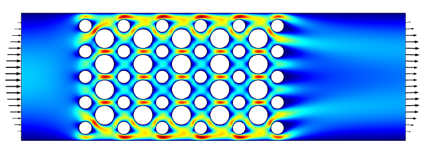
Image of water flow around obstructions in a reactor.
Once the flow field is computed, we also want to plot and compute the following:
- Residence time distribution function
- Cumulative distribution function
- Mean residence time
- Variance
To solve for these quantities, it is most convenient to use a Lagrangian formulation to trace a computational particle as it moves with the fluid, rather than using the Eulerian formulation used to solve for the flow field. For this reason, as well as the built-in features available for conveniently evaluating particle tracing results, we will address this using the capabilities of the Particle Tracing Module.
Using the Particle Tracing Functionality in the COMSOL® Software
The use of the Particle Tracing Module to trace streamlines of the flow field, and to integrate along these streamlines, is covered in this Learning Center article. Along with those methods, there are additional techniques to bookkeep the particles in the flow, as described in this previous blog post.
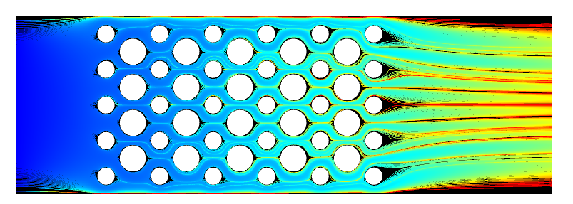
Streamlines of the flow, colored by the time it takes a particle traced along the flow to reach that point.
The results shown above visualize the time of a computational particle being traced along the streamlines. The residence time distribution and the cumulative distribution at the outlet are shown in the plots below. It’s additionally possible to extract scalar values such as the mean residence time and variance, as described in the Learning Center article mentioned above.
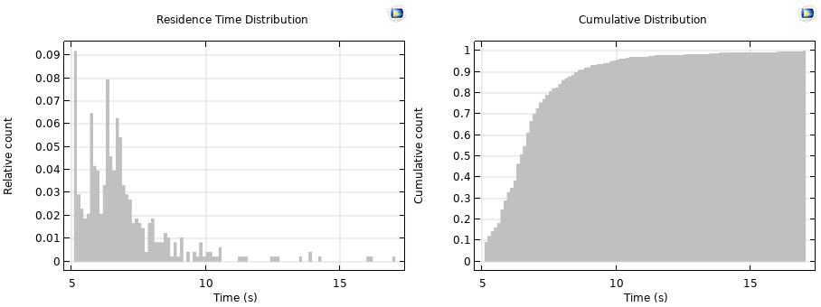
Plots of residence time distribution (left) and cumulative distribution (right).
Closing Remarks
Here we have only traced the streamlines of the flow field, but the functionality of the Particle Tracing Module has wide-ranging applications for augmenting the analysis of flow fields. It is particularly useful, as its name implies, when we want to consider actual particles in the flow, in which case we can also include the effects of:
- Particle inertia
- A distribution of particle sizes
- Changing of size/mass during transit
- Arbitrary additional governing ODEs solved with the moving particle
- Forces on the particles
- Drag
- Turbulent dispersion
- Lift
- Gravity
- Centrifugal
- Electric
- Dielectrophoretic
- Magnetic
- Magnetophoretic
- Brownian (molecular diffusion)
- Thermophoretic
- Acoustophoretic
- Particle–particle interaction
- Coupled fluid-particle interactions
For an overview of the other formulations that are available, see this previous blog post.
Next Step
Learn more about the specialized features and functionality in the Particle Tracing Module by clicking the button below.