A question we get asked all of the time is: “Which of the COMSOL products should be used for modeling a particular electromagnetic device or application?” In addition to the capabilities of the core package of the COMSOL Multiphysics® software, there are currently six modules within the “Electromagnetic Modules” branch of our product tree, and another six modules spread throughout the remaining product structure that address various forms of Maxwell’s equations coupled to other physics. Let’s take a look through these and see what they offer.
Note: This blog post was originally published on September 10, 2013. It has since been updated with additional information and examples.
Computational Electromagnetics: Maxwell’s Equations
Maxwell’s equations relate the electric charge density, ![]() ; electric field,
; electric field, ![]() ; electric displacement field,
; electric displacement field, ![]() ; and current,
; and current, ![]() ; as well as the magnetic field intensity,
; as well as the magnetic field intensity, ![]() , and the magnetic flux density,
, and the magnetic flux density, ![]() :
:
|
\nabla \cdot \mathbf{D} = \rho
|
\nabla \cdot \mathbf{B} = 0
|
|
\nabla \times \mathbf{E} = -\frac{\partial}{\partial t} \mathbf{B}
|
\nabla \times \mathbf{H} = \mathbf{J} + \frac{\partial}{\partial t} \mathbf{D}
|
To solve these equations, we need a set of boundary conditions, as well as material constitutive relations that relate the ![]() to the
to the ![]() field, the
field, the ![]() to the
to the ![]() field, and the
field, and the ![]() to the
to the ![]() field. Under varying assumptions, these equations are solved, and coupled to the other physics, in the different modules within the COMSOL product suite.
field. Under varying assumptions, these equations are solved, and coupled to the other physics, in the different modules within the COMSOL product suite.
Note: Most of the equations presented here are shown in an abbreviated form to convey the key concepts. To see the full form of all governing equations, and to see all of the various constitutive relationships available, please consult the Product Documentation.
Let’s start off with a few concepts…
Steady State, Time, or Frequency Domain?
When solving Maxwell’s equations, we try to make as many assumptions as are reasonable and correct, with the purpose of easing our computational burden. Although Maxwell’s equations can be solved for any arbitrary time-varying inputs, we can often reasonably assume that the inputs, and computed solutions, are either steady-state or sinusoidally time-varying. The former is also often referred to as the DC (direct current) case, and the latter is often to as the AC (alternating current), or frequency domain, case.
The steady-state (DC) assumption holds if the fields do not vary at all in time, or vary so negligibly as to be unimportant. That is, we would say that the time-derivative terms in Maxwell’s equations are zero. For example, if your device is connected to a battery (which might take hours or longer to drain appreciably), this would be a very reasonable assumption to make. More formally, we would say that: ![]() , which immediately omits two terms from Maxwell’s equations.
, which immediately omits two terms from Maxwell’s equations.
The frequency-domain assumption holds if the excitations on the system vary sinusoidally and if the response of the system also varies sinusoidally at the same frequency. Another way of saying this is that the response of the system in linear. In such cases, rather than solving the problem in the time domain, we can solve in the frequency domain using the relationship: ![]() , where
, where ![]() is the space- and time-varying field;
is the space- and time-varying field; ![]() is a space-varying, complex-valued field; and
is a space-varying, complex-valued field; and ![]() is the angular frequency. Solving Maxwell’s equations at a set of discrete frequencies is very computationally efficient as compared to the time domain, although the computational requirements grow in proportion to the number of different frequencies being solved for (with some caveats that we will discuss later).
is the angular frequency. Solving Maxwell’s equations at a set of discrete frequencies is very computationally efficient as compared to the time domain, although the computational requirements grow in proportion to the number of different frequencies being solved for (with some caveats that we will discuss later).
Solving in the time domain is needed when the solution varies arbitrarily in time or when the response of the system is nonlinear (although even to this, there are exceptions, which we will discuss). Time-domain simulations are more computationally challenging than steady-state or frequency-domain simulations because their solution times increase in proportion to how long the time span of interest is, and the nonlinearities that are being considered. When solving in the time domain, it is helpful to think in terms of the frequency content of your input signal, especially the highest frequency that is present and significant.
Electric Fields, Magnetic Fields, or Both?
Although we can solve Maxwell’s equations for both the electric and the magnetic fields, it is often sufficient to neglect one, or the other, especially in the DC case. For example, if the currents are quite small in magnitude, the magnetic fields are going to be small. Even in cases where the currents are high, we might not actually concern ourselves about the resultant magnetic fields. On the other hand, sometimes there is solely a magnetic field, but no electric field, as in the case of a device composed only of magnets and magnetic materials.
In the time- and frequency domains, though, we have to be a bit more careful. The first quantity we will want to check here is the skin depth of the materials in our model. The skin depth of a metallic material is usually approximated as ![]() , where
, where ![]() is the permeability and
is the permeability and ![]() is the conductivity. If the skin depth is much larger than the characteristic size of the object, then it is reasonable to say that skin depth effects are negligible and one can solve solely for the electric fields. However, if the skin depth is equal to, or smaller than, the size of the object, then inductive effects are important and we need to consider both the electric and magnetic fields. It’s good to do a quick check of the skin depth before starting any modeling.
is the conductivity. If the skin depth is much larger than the characteristic size of the object, then it is reasonable to say that skin depth effects are negligible and one can solve solely for the electric fields. However, if the skin depth is equal to, or smaller than, the size of the object, then inductive effects are important and we need to consider both the electric and magnetic fields. It’s good to do a quick check of the skin depth before starting any modeling.
As one increases the excitation frequency, it is also important to know the first resonance of the device. At this fundamental resonant frequency, the energy in the electric fields and magnetic fields are exactly in balance, and we would say that we are in the high-frequency regime. Although it is generally difficult to estimate the resonant frequency, a good rule of thumb is to compare the characteristic object size, ![]() , to the wavelength,
, to the wavelength, ![]() . If the object size approaches a significant fraction of the wavelength,
. If the object size approaches a significant fraction of the wavelength, ![]() , then we are approaching the high-frequency regime. In this regime, power flows primarily via radiation through dielectric media, rather than via currents within conductive materials. This leads to a slightly different form of the governing equations. Frequencies significantly lower than the first resonance are often termed the low-frequency regime.
, then we are approaching the high-frequency regime. In this regime, power flows primarily via radiation through dielectric media, rather than via currents within conductive materials. This leads to a slightly different form of the governing equations. Frequencies significantly lower than the first resonance are often termed the low-frequency regime.
Let’s now look at how these various different assumptions are applied to Maxwell’s equations, and give us different sets of equations to solve, and then see which modules we would need to use for each.
Steady-State Electric Field Modeling
Under the assumption of steady-state conditions, we can further assume that we are dealing solely with conductive materials, or perfectly insulative materials. In the former case, we can assume that current flows in all domains, and Maxwell’s equations can be rewritten as:
\nabla \cdot \left( – \sigma \nabla V \right ) = 0
This equation solves for the electric potential field, ![]() , which gives us the electric field,
, which gives us the electric field, ![]() , and the current,
, and the current, ![]() . This equation can be solved with the core COMSOL Multiphysics package and is solved in the introductory example to the software. The AC/DC Module and the MEMS Module extend the capabilities of the core package, for example, by offering terminal conditions that simplify model setup and boundary conditions for modeling of relatively thin conductive and insulative regions, as well as separate physics interfaces for modeling the current flow solely through geometrically thin, possibly multilayered, structures.
. This equation can be solved with the core COMSOL Multiphysics package and is solved in the introductory example to the software. The AC/DC Module and the MEMS Module extend the capabilities of the core package, for example, by offering terminal conditions that simplify model setup and boundary conditions for modeling of relatively thin conductive and insulative regions, as well as separate physics interfaces for modeling the current flow solely through geometrically thin, possibly multilayered, structures.
On the other hand, under the assumption that we are interested in the electric fields in perfectly insulating media, with material permittivity, ![]() , we can solve the equation:
, we can solve the equation:
\nabla \cdot \left( – \epsilon \nabla V \right ) = 0
This computes the electric field strength in the dielectric regions between objects at different electric potentials. This equation can also be solved with the core COMSOL Multiphysics package, and again, the AC/DC and MEMS modules extend the capabilities via, for example, terminal conditions, boundary conditions for modeling thin dielectric regions, and thin gaps in dielectric materials. Furthermore, these two products additionally offer the boundary element formulation, which solves the same governing equation, but has some advantages for models composed of just wires and surfaces, as discussed in this previous blog post.
Time- and Frequency-Domain Electric Field Modeling
As soon as you want to model time-varying electric fields, there will be both conduction and displacement currents, and you will want to use either the AC/DC Module or MEMS Module. The equations here are only slightly different from the first equation, above, and in the time-domain case, are written as:
\nabla \cdot \left( \mathbf{J_c +J_d} \right ) = 0
This transient equation solves for both conduction currents, ![]() , and displacement currents,
, and displacement currents, ![]() . This is appropriate to use when the source signals are nonharmonic and you wish to monitor system response over time. You can see an example of this in the Transient Modeling of a Capacitor in a Circuit model.
. This is appropriate to use when the source signals are nonharmonic and you wish to monitor system response over time. You can see an example of this in the Transient Modeling of a Capacitor in a Circuit model.
In the frequency domain, we can instead solve the stationary equation:
\nabla \cdot \left( – \left( \sigma + j \omega \epsilon \right) \nabla V \right ) = 0
The displacement currents in this case are ![]() . An example of the usage of this equation is the Frequency Domain Modeling of a Capacitor model.
. An example of the usage of this equation is the Frequency Domain Modeling of a Capacitor model.
Magnetic Field Modeling with the AC/DC Module
Modeling of magnetic fields, in the steady-state, time-domain, or low-frequency regime, is addressed within the AC/DC Module.
For models that have no current flowing anywhere, such as models of magnets and magnetic materials, it is possible to simplify Maxwell’s equations and solve for ![]() , the magnetic scalar potential:
, the magnetic scalar potential:
\nabla \cdot \left( – \mu \nabla V_m \right ) = 0
This equation can be solved using either the finite element method or the boundary element method.
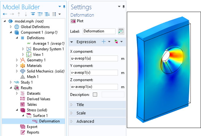
Once there are steady-state currents in the model, we must instead solve for ![]() , the magnetic vector potential.
, the magnetic vector potential.
\nabla \times \left( \mu ^ {-1} \nabla \times \mathbf{A} \right)= \mathbf{J}
This magnetic vector potential is used to compute ![]() , and the current,
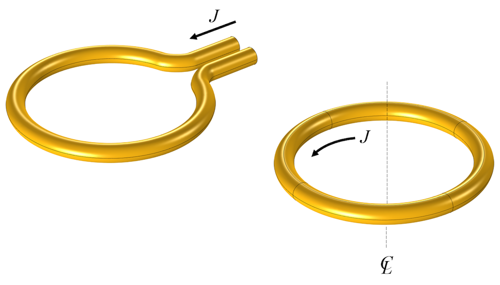
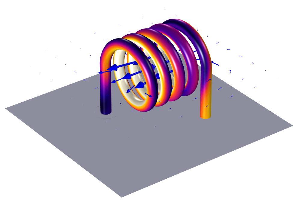
, and the current, ![]() , can be either imposed or simultaneously computed via augmenting with the previous equation for the electric scalar potential and current. A typical example of such a case is the magnetic field of a Helmholz coil.
, can be either imposed or simultaneously computed via augmenting with the previous equation for the electric scalar potential and current. A typical example of such a case is the magnetic field of a Helmholz coil.
As we move to the time domain, we solve the following equation:
\nabla \times \left( \mu ^ {-1} \nabla \times \mathbf{A} \right)=- \sigma \frac{ \partial \mathbf{A}}{\partial t}
where ![]() .
.
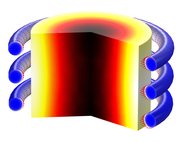
This equation considers solely the conduction currents and induced currents, but not the displacement currents. This is reasonable if the power transfer is primarily via conduction and not radiation. One strong motivation behind solving this equation is if there are material nonlinearities, such as a B-H nonlinear material, as in this example of an E-core transformer. It should be noted, though, that there are alternative ways of solving B-H nonlinear materials via an effective H-B curve approach.
As we move into the frequency domain, the governing equation becomes:
\nabla \times \left( \mu ^ {-1} \nabla \times \mathbf{A} \right) = -\left( j \omega \sigma – \omega^2 \epsilon \right) \mathbf{A}
Note that this equation considers both conduction currents, ![]() , and displacement currents,
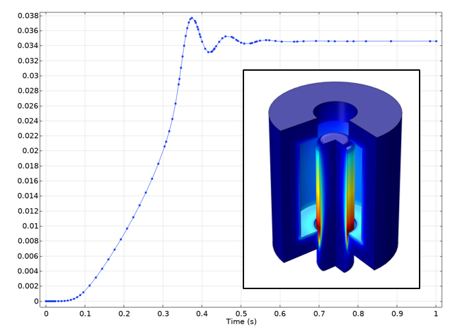
, and displacement currents, ![]() , and is starting to look quite similar to a wave equation. In fact, this equation can solve up to and around the resonance of a structure under the assumption that there is negligible radiation, as demonstrated in this example: Modeling of a 3D Inductor.
, and is starting to look quite similar to a wave equation. In fact, this equation can solve up to and around the resonance of a structure under the assumption that there is negligible radiation, as demonstrated in this example: Modeling of a 3D Inductor.
For a more complete introduction to the usage of the above sets of equations for magnetic field modeling, also see our lecture series on electromagnetic coil modeling.
It is also possible to mix the magnetic scalar potential and vector potential equations, and this has applications for modeling of motors and generators.
In addition to the above static, transient, and frequency-domain equations in terms of the magnetic vector potential and scalar potential, there also exists a separate formulation in terms of the magnetic field, which is appropriate for modeling of superconducting materials, as in this example of a superconducting wire.
Wave Equation Modeling in the Frequency and Time Domains with the RF or Wave Optics Modules
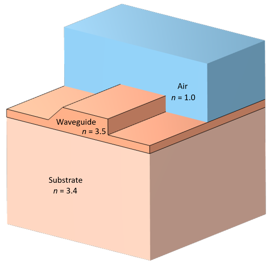
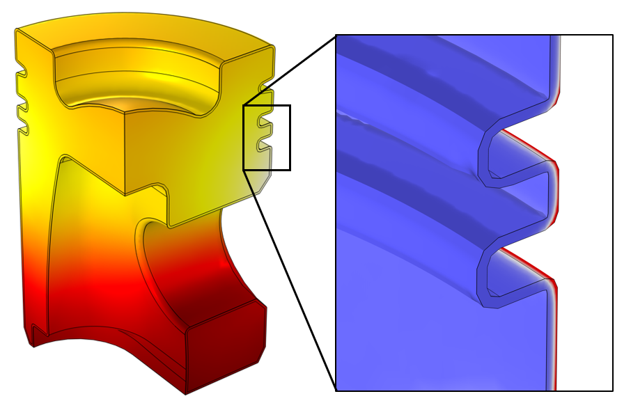
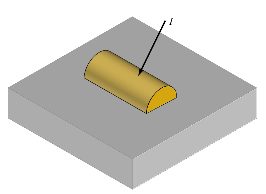
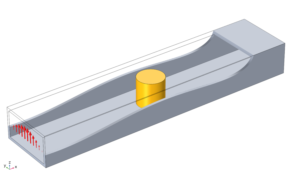
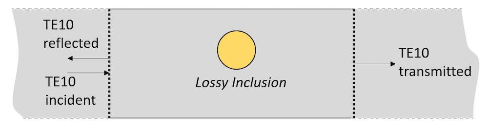
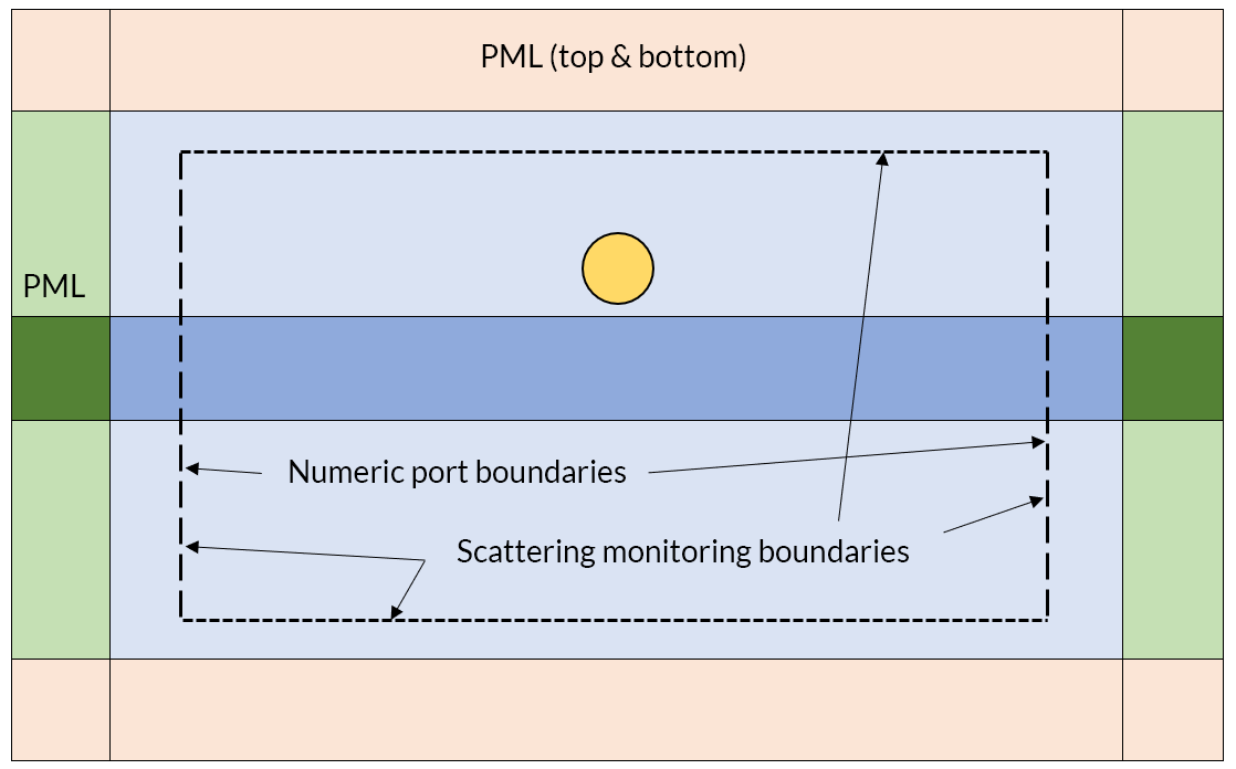
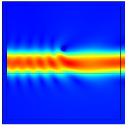
As we get into the high-frequency regime, the electromagnetic fields become wave-like in nature, as in the modeling of antennas, microwave circuits, optical waveguides, microwave heating, and scattering in free space, as well as scattering from an object on a substrate, and we solve a slightly different form of Maxwell’s equations in the frequency domain:
\nabla \times \left( \mu_r ^ {-1} \nabla \times \mathbf{E} \right) -\omega^2 \epsilon_0 \mu_0 \left(\epsilon_r – j \sigma/\omega \epsilon_0 \right) \mathbf{E} = 0
This equation is written in terms of the electric field, ![]() , and the magnetic field is computed from:
, and the magnetic field is computed from: ![]() . It can be solved either at a specified set of frequencies, or as an eigenfrequency problem, which directly solves for the resonant frequency of the device. Examples of eigenfrequency analysis include several benchmarks of closed cavities, coils, and Fabry–Perot cavities, and such models compute both resonant frequencies and quality factor.
. It can be solved either at a specified set of frequencies, or as an eigenfrequency problem, which directly solves for the resonant frequency of the device. Examples of eigenfrequency analysis include several benchmarks of closed cavities, coils, and Fabry–Perot cavities, and such models compute both resonant frequencies and quality factor.
When solving for the system response over a range of specified frequencies, one can directly solve at a set of discrete frequencies, in which case the computational cost scales linearly with number of specified frequencies. One can also instead exploit hardware parallelism on both single computers and clusters to parallelize and speed up solutions. There are also Frequency-Domain Modal and Adaptive Frequency Sweep (also called Asymptotic Waveform Evaluation) solvers that accelerate the solutions to some types of problems, as introduced in a general sense in this blog post, and demonstrated in this waveguide iris filter example.
If you’re instead solving in the time domain with the RF or Wave Optics modules, then we solve an equation that looks very similar to the earlier equation from the AC/DC Module:
\nabla \times \left( \mu_r ^ {-1} \nabla \times \mathbf{A} \right)+ \mu_0 \sigma \frac{ \partial \mathbf{A}}{\partial t} +\mu_0 \frac{ \partial}{\partial t} \left( \epsilon_0 \epsilon_r \frac{ \partial \mathbf{A}}{\partial t} \right) = 0
This equation again solves for the magnetic vector potential, but includes both first and second derivatives in time, thus considering both conduction and displacement currents. It has applicability in modeling of optical nonlinearities, dispersive materials, and signal propagation. Time domain results can also be converted into the frequency domain via a Fast Fourier Transform solver, as demonstrated in this example.
The computational requirements for these equations, in terms of memory, also are a concern. The device of interest, and the space around it, are discretized via the finite element mesh, and this mesh must be fine enough to resolve the wave. That is, at a minimum, the Nyquist criterion must be fulfilled. In practice, this means that a domain size of about 10 x 10 x 10 wavelengths in size (regardless of the operating frequency) represents about the upper limit of what is addressable on a desktop computer with 64 GB of RAM. As the domain size increases (or the frequency increases), the memory requirements will grow in proportion to the number of cubic wavelengths being solved for. This means that the above equation is well suited for structures that have characteristic size roughly no larger that 10 times the wavelength at the highest operating frequency of interest. There are, however, two ways to get around this limit.
One approach for solving for the wave-like fields around an object much smaller than the wavelength is the Time Explicit formulation. This solves a different form of the time-dependent Maxwell’s equations that can be solved using much less memory. It is primarily meant for linear material modeling, and is attractive in some cases such as for computing wideband scattering off an object in a background field.
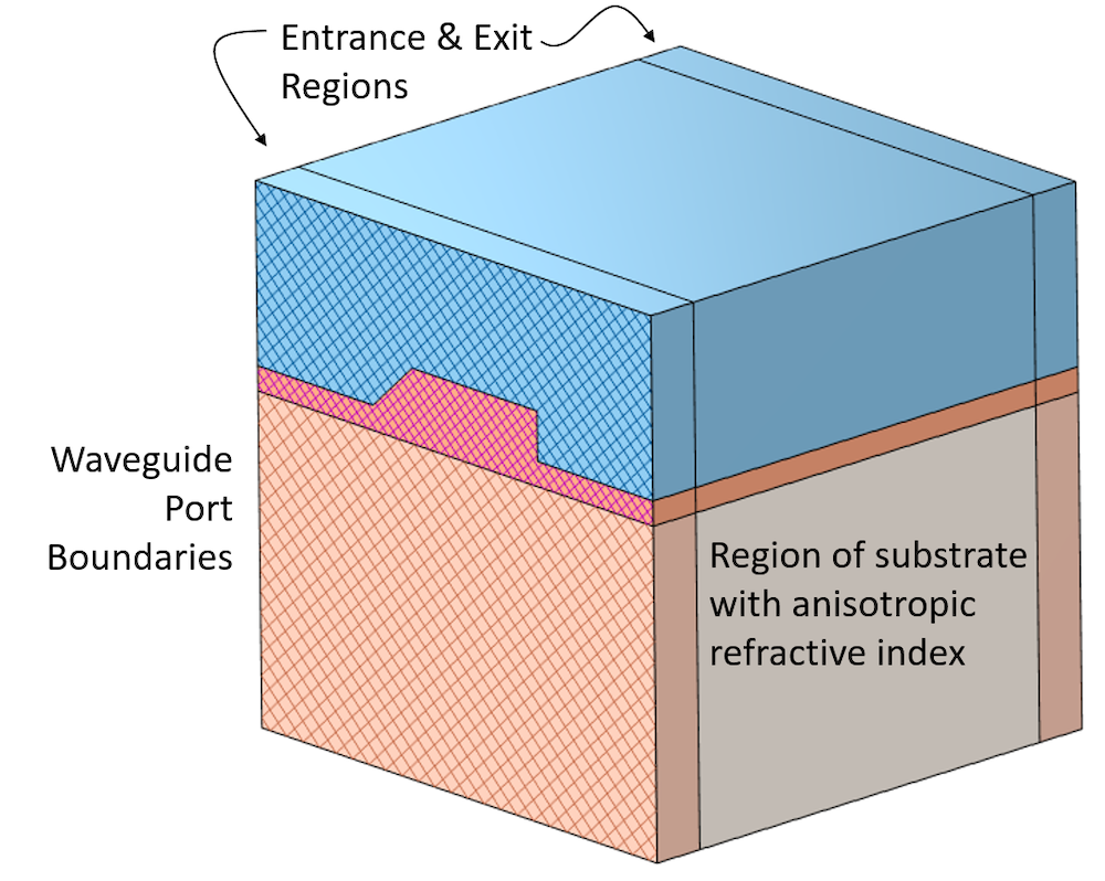
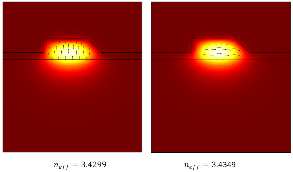
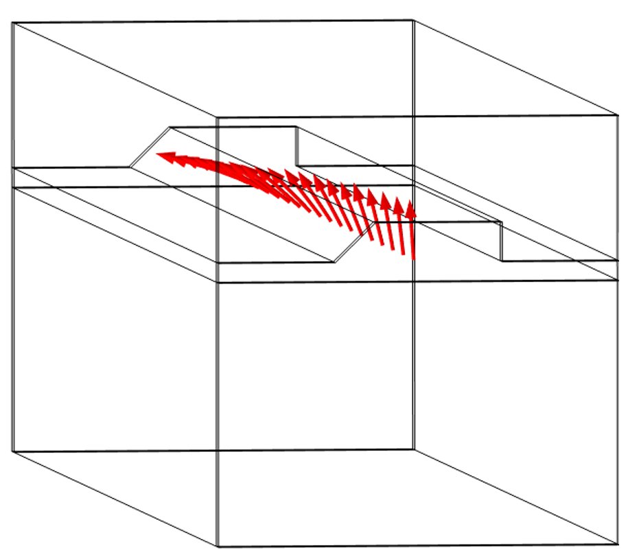
Another alternative exists for certain types of optical waveguiding structures, solved in the frequency domain, where it is known that the electric field varies quite slowly in the direction of propagation. In such cases, the beam envelopes method in the Wave Optics Module becomes quite attractive. This interface solves the equation:
\left( \nabla – i \nabla \phi \right) \times \mu_r ^ {-1} \left( \left( \nabla – i \nabla \phi \right) \times \mathbf{E_e} \right) -\omega^2 \epsilon_0 \mu_0 \left(\epsilon_r – j \sigma/\omega \epsilon_0 \right) \mathbf{E_e} = 0
Where the electric field is ![]() and
and ![]() is the envelope of the electric field.
is the envelope of the electric field.
The additional field, ![]() , is a so-called phase function that must be known, at least approximately, and specified as an input. Luckily, for many optical waveguiding problems, this is indeed the case. It is possible to solve for either just one, or two, such beam envelope fields at the same time. The advantage of this approach, when it can be used, is that the memory requirements are far lower than for the full-wave equation presented at the beginning of this section. Other examples of its usage include models of a directional coupler as well as modeling of self-focusing in optical glass.
, is a so-called phase function that must be known, at least approximately, and specified as an input. Luckily, for many optical waveguiding problems, this is indeed the case. It is possible to solve for either just one, or two, such beam envelope fields at the same time. The advantage of this approach, when it can be used, is that the memory requirements are far lower than for the full-wave equation presented at the beginning of this section. Other examples of its usage include models of a directional coupler as well as modeling of self-focusing in optical glass.
Deciding Between the AC/DC Module, RF Module, and Wave Optics Module
The dividing line between the AC/DC Module and the RF Module is a bit of a fuzzy line. It’s helpful to ask yourself a few questions:
- Are the devices I’m working with radiating significant amounts of energy? Am I interested in computing resonances? If so, the RF Module is more appropriate.
- Are the devices much smaller than the wavelength at the highest operating wavelength? Am I primarily interested int the magnetic fields? If so, the AC/DC Module is more appropriate.
If you’re right at the line between these, then it can even be reasonable to have both products in your suite of modules.
Deciding between the RF Module and Wave Optics Module involves asking yourself about your applications. Although there is a lot of overlap in functionality in terms of the full-wave form of Maxwell’s equations in the time and frequency domains, there are some small differences in the boundary conditions. There are so-called Lumped Port and Lumped Element boundary conditions, applicable for microwave device modeling, which are solely part of the RF Module. Also keep in mind that only the Wave Optics Module contains the beam envelopes formulation.
As far as material properties, the two products come with different libraries of materials: The RF Module offers a suite of common dielectric substrates, while the Wave Optics Module includes refractive indices of over a thousand different materials in the optical and IR band. For more details on this, and the other available libraries of materials, see this blog post. Of course, if you have specific questions about your device modeling needs, contact us.
A summary of the approximate dividing lines between these modules is given in the figure below.
![A graph comparing the RF, AC/DC, and Wave Optics modules for electromagnetics analyses.]()
Ray Tracing with the Ray Optics Module
If you are modeling devices many thousands of times the wavelength in size, then it is no longer possible to resolve the wavelength via a finite element mesh. In such cases, we also offer a geometrical optics approach in the Ray Optics Module. This approach does not directly solve Maxwell’s equations, but instead traces rays through the modeling space. This approach requires only that reflective surfaces and dielectric domains, but not uniform free space, be meshed. It is applicable for modeling of lenses, telescopes, large laser cavities, as well as structural-thermal-optical performance (STOP) analysis. It can even be combined with the output of a full-wave analysis, as demonstrated in this tutorial model.
Multiphysics Modeling
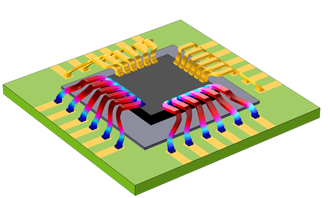
In addition to solving Maxwell’s equations on their own, one of the core strengths of COMSOL Multiphysics is solving problems where there are couplings between several physics. One of the most common is the coupling between Maxwell’s equations and temperature, wherein the rise in temperature affects the electrical (as well as the thermal) properties. For an overview of the ways in which these kinds of electrothermal problems can be addressed, please see this blog post.
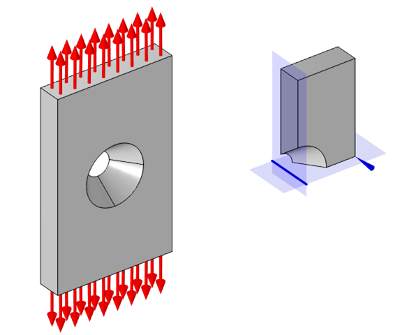
It is also common to couple structural deformations to electric and magnetic fields. Sometimes, this just involves deformation, but sometimes, this also involves piezoelectric, piezoresistive, or magnetostrictive material response, or even a stress-optical response. The MEMS Module has a dedicated user interface for electrostatically actuated resonators, wherein an applied electric field biases a device. Structural contact and the flow of current between contacting parts can also be considered in the context of electric currents modeling.
Beyond just temperature and deformation, though, you can also couple Maxwell’s equations for electric current to chemical processes, as addressed by the Electrochemistry, Batteries & Fuel Cells, Electrodeposition, and Corrosion modules. In the Plasma Module, you can even couple to plasma chemistry, and with the Particle Tracing Module, you can trace charged particles through electric and magnetic fields. Lastly (for now!) our Semiconductor Module solves for charge transport using the drift-diffusion equations. Each of these modules is a topic in and of itself, so we won’t try to address them all right here.
Of course, if you would like to discuss any of these modules in greater depth, and find out how it is applicable to your device of interest, don’t hesitate to contact us via the button below.
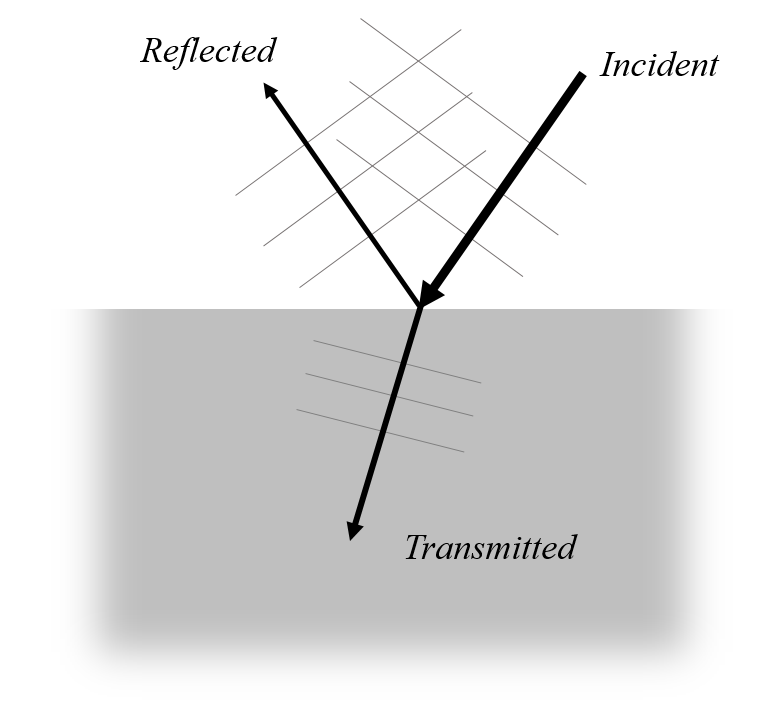
 ) and transmitted (
 ) light relative to the surface normal in terms of the refractive indices,
  and
and  , of the two materials:
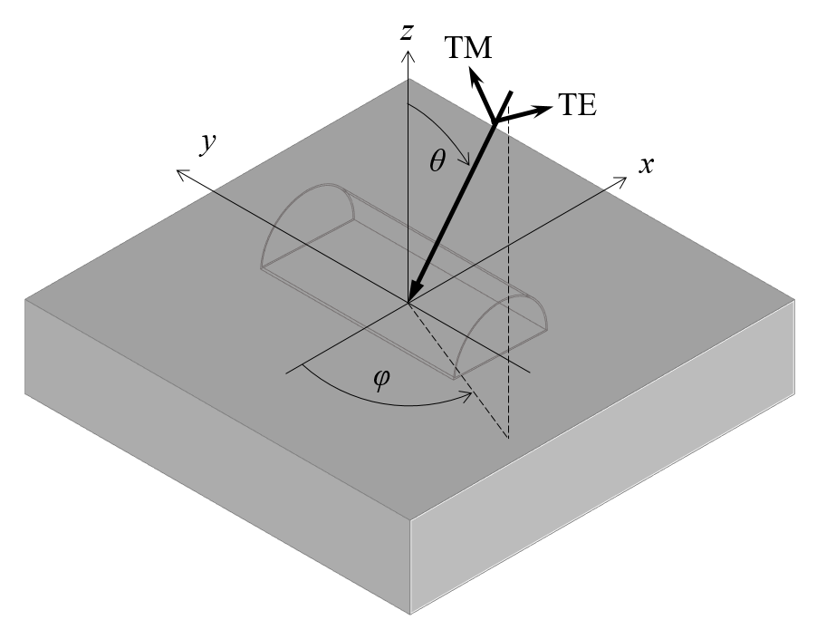
 is propagating in the negative z direction, we define the angle of incidence
  as the angle from the z-axis, and the angle
  as the rotation about the z-axis starting from the negative x-axis, as shown in the figure above. This lets us define the k-vectors of the incident beam as:
 , is similar to the incident beam, but of opposite sign for the z-component.
  and
and  , the components of the electric field of the incident beam are:
 , and of the other side of the interface, the field is
  , with components:

 ; electric field,
  ; electric displacement field,
  ; and current,
  ; as well as the magnetic field intensity,
  , and the magnetic flux density,
  :
: , which immediately omits two terms from Maxwell’s equations.
  , where
  is the space- and time-varying field;
  is a space-varying, complex-valued field; and
  is the angular frequency. Solving Maxwell’s equations at a set of discrete frequencies is very computationally efficient as compared to the time domain, although the computational requirements grow in proportion to the number of different frequencies being solved for (with some caveats that we will discuss later).
 , where
  is the permeability and
  is the conductivity. If the skin depth is much larger than the characteristic size of the object, then it is reasonable to say that skin depth effects are negligible and one can solve solely for the electric fields. However, if the skin depth is equal to, or smaller than, the size of the object, then inductive effects are important and we need to consider both the electric and magnetic fields. It’s good to do a quick check of the skin depth before starting any modeling.
  , to the wavelength,
  . If the object size approaches a significant fraction of the wavelength,
  , then we are approaching the high-frequency regime. In this regime, power flows primarily via radiation through dielectric media, rather than via currents within conductive materials. This leads to a slightly different form of the governing equations. Frequencies significantly lower than the first resonance are often termed the low-frequency regime.
  , which gives us the electric field,
  , and the current,
  . This equation can be solved with the core
  , we can solve the equation:
 , and displacement currents,
  . This is appropriate to use when the source signals are nonharmonic and you wish to monitor system response over time. You can see an example of this in the
  . An example of the usage of this equation is the
  , the magnetic scalar potential:
 , the magnetic vector potential.
  , and the current,
  .
. , and displacement currents,
  , and is starting to look quite similar to a wave equation. In fact, this equation can solve up to and around the resonance of a structure under the assumption that there is negligible radiation, as demonstrated in this example:
  . It can be solved either at a specified set of frequencies, or as an eigenfrequency problem, which directly solves for the resonant frequency of the device. Examples of eigenfrequency analysis include several benchmarks of
  and
and  is the envelope of the electric field.
 , is a so-called phase function that must be known, at least approximately, and specified as an input. Luckily, for many optical waveguiding problems, this is indeed the case. It is possible to solve for either just one, or two, such beam envelope fields at the same time. The advantage of this approach, when it can be used, is that the memory requirements are far lower than for the full-wave equation presented at the beginning of this section. Other examples of its usage include models of a
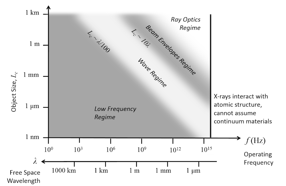
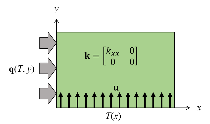
 , in the absence of volumetric heating but with a convective term,
  , as follows:
 is the material density;
  the specific heat; and
  is the thermal conductivity, which in this case is a diagonal matrix of the form:
 , and we will set the y-component of the diagonal thermal conductivity tensor to zero,
  . Now the above equation reduces to:
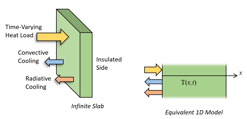
 -th root. This is the
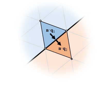
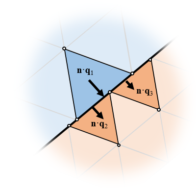
 . At boundaries between elements, the FEM automatically (that is, without needing any user input or additional internal equations) enforces the condition that
  , where
  is the normal vector to the boundary between elements. That is, the standard FEM naturally enforces the continuity of the fields and balances fluxes. Do keep in mind that, regardless of this, you will always need to do a
 represents a heat load; and the denominator of the above equation,
  , represents a system thermal conductance.
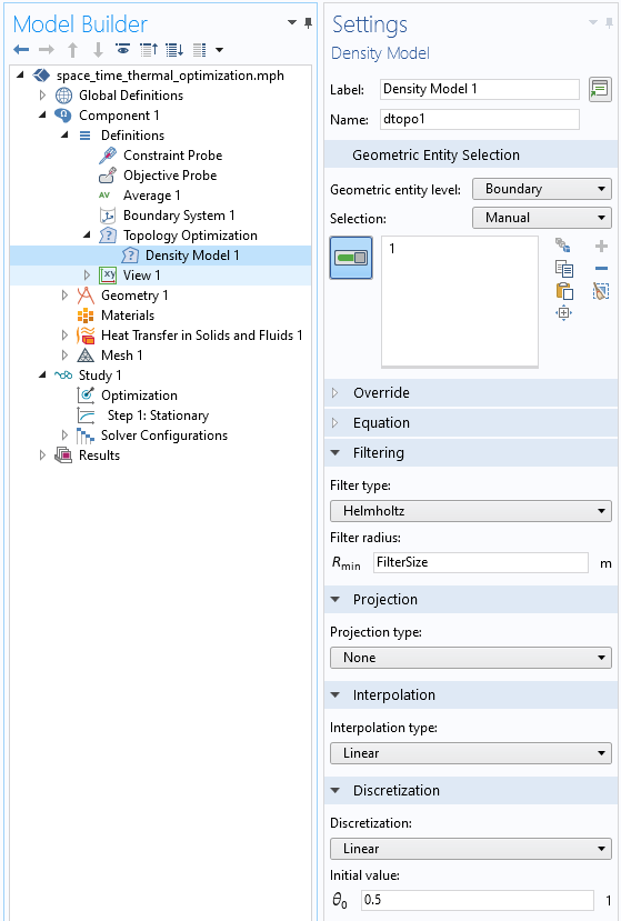
 operating system, since we will be using the Application Builder functionality. Click on the Application Builder button in the ribbon, or use the keyboard shortcut Control+Shift+A, and you’ll be brought to the interface shown below. The one task that we will do here is add a new method with the Methods branch. Give it a name, e.g.,


 , and the temperature fields,
  , will be nonzero.


 , and a magnetic field,
  , at a velocity,
  . The total force on a particle, of charge
  , is:
, is: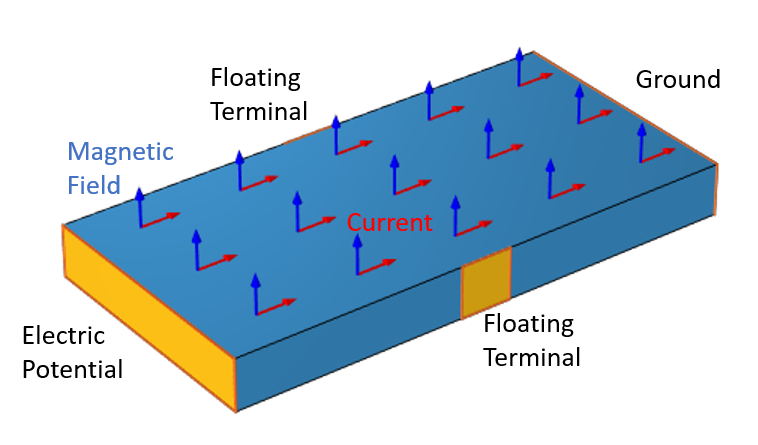
 , and
, and  , the Hall coefficient:
 is negligible and can be ignored.
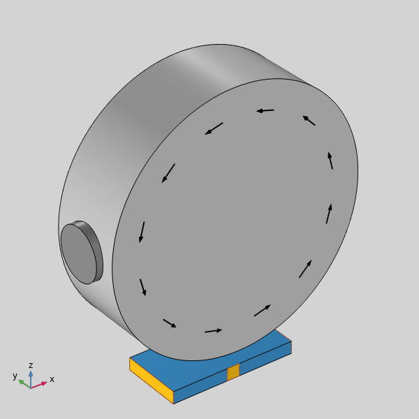
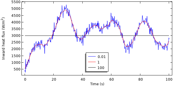
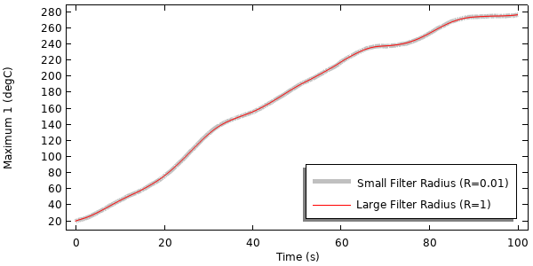
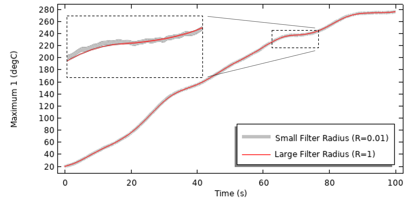
 is the input data and
  is the filtered data.
 , which we will call the filter radius.